DLM demo no 1

Generate synthetic and ideal data and fit a DLM smoother. The command dlmgensys generates system evolution matrix G and obs operator F. We use local level and trend model with 12 seasons.

[G,F] = dlmgensys(struct('order',1,'fullseas',1,'ns',12));
% p = number of data sets = 1,
% m = number of internal states = 13
[p,m] = size(F);

Generate data.

t = (1:1:(6*12))'; % time
n = length(t);
s = 0.1; % obs error std
V = ones(n,p)*s; % V is matrix of std's
x0 = [0;0.001;sin((1:11)/12*pi*2)']; % initial state
C0 = 0.02*eye(m)*s^2; % initial state uncertainty
W = zeros(m); % "model error"
W(1,1) = 0.000002^2;
W(2,2) = 0.002.^2;
W(3,3) = 0.02.^2;

Observations are generated using the state space recursion.

y = zeros(n,1);
x = x0;
for i=1:n
  y(i) = F*x + randn(1,1)*s;
  x = G*x + randn(m,1).*sqrt(diag(W));
end

Function dlmsmo calculates the estimated states using Kalman smoother.

out = dlmsmo(y,F,V,x0,G,W,C0);
x0 = out.x(:,1); % save smoothed estimate of x0

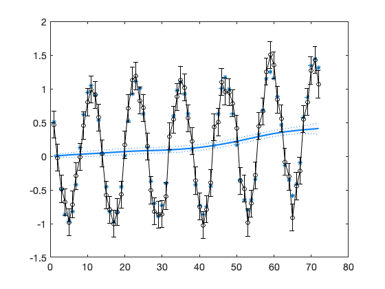
Plot observations and the fitted level with 95% (time wise) confidence bands.

figure(1); clf
plot(t,out.yhat,'*')
hold on
confband(t,out.x(1,:)',out.xstd(:,1));
errorbar(t,y,2*V,'ok-')
hold off

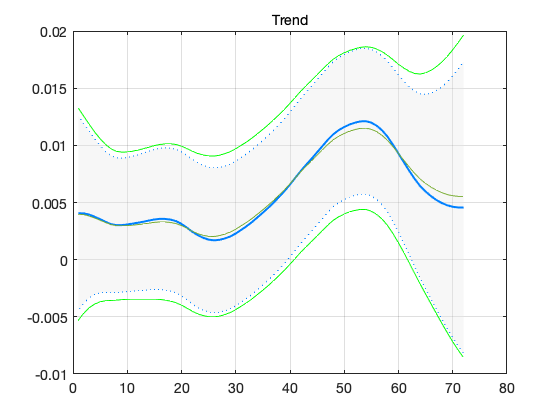
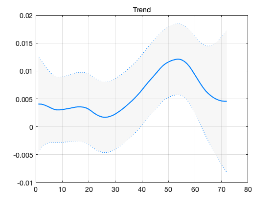
figure(2); clf
confband(t,out.x(2,:)',out.xstd(:,2)); grid; title('Trend')

MCMC

Gibbs sampling for the variance parameters using conjugate prior distributions. This takes some time.

nsimu = 1000;
chain = zeros(nsimu,4);
W0 = W; % prior W
n0 = 5; % prior weight
V0 = s;
nv0 = 10;
doplot = 1;
plotint = 100;

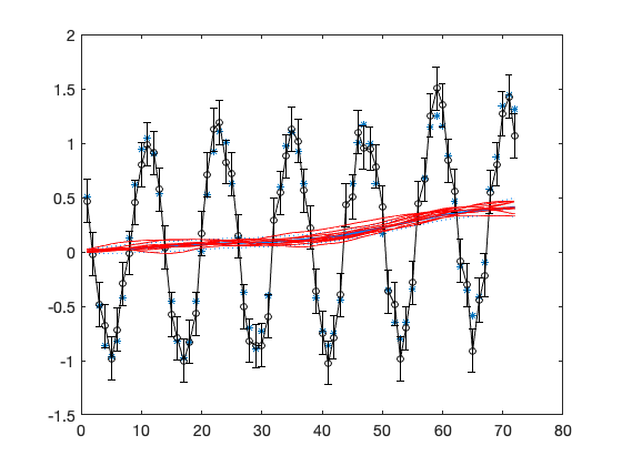
hw = waitbar(0,'MCMC running, please wait');
for isimu = 1:nsimu
  waitbar(isimu/nsimu,hw);
  % Gibbs step for variance parameters
  % residual std for V, conjugate distribution is inverse chi squared
  sigV = sqrt(invchir(1,1,n+nv0,(out.ssy+V0.^2*nv0)/(n+nv0)));
  V = ones(n,p)*sigV;
  out = dlmsmo(y,F,V,x0,G,W,C0); % recalculate with new V
  % variances in diag(W)
  c = zeros(1,3); % fit 3 first variances
  for i=1:3
    c(i) = invchir(1,1,n+n0-1,(W0(i,i).*n0+out.ss(i))./(n+n0-1));
    W(i,i) = c(i);
    out = dlmsmo(y,F,V,x0,G,W,C0);  % recalculate smoother
  end
  chain(isimu,:) = [sigV,sqrt(c(1:3))];
  if doplot & (isimu/plotint == fix(isimu/plotint))
    % plot every plotint'th MCMC sampled state
    figure(1);
    hold on
    plot(t,out.xr(1,:),'-r')
    hold off
  end
end
close(hw);

figure(3); clf
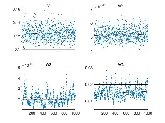
mcmcplot(chain,[],{'V','W1','W2','W3'});
hold on
subplot(2,2,1); h=hline(s);set(h,'linestyle','-','linewidth',2)
subplot(2,2,2); h=hline(sqrt(W0(1,1)));set(h,'linestyle','-','linewidth',2)
subplot(2,2,3); h=hline(sqrt(W0(2,2)));set(h,'linestyle','-','linewidth',2)
subplot(2,2,4); h=hline(sqrt(W0(3,3)));set(h,'linestyle','-','linewidth',2)
hold off

V = ones(n,p)*sqrt(mean(chain(:,1).^2));
for i=1:3;  W(i,i) = mean(chain(:,i+1).^2); end

out = dlmsmo(y,F,V,x0,G,W,C0);

Add estimated over the initial trend.

figure(2);
ind = 2; %
xxx = out.x(ind,:)';
hold on
plot(t,xxx)
plot(t,xxx-2*out.xstd(:,ind),'g-')
plot(t,xxx+2*out.xstd(:,ind),'g-')
hold off

Published with MATLAB® R2018b